Getting started with rcrisp

What is `rcrisp`?

rcrisp automates the morphological delineation of riverside urban areas following a method developed by Forgaci (2018, pp. 88–89). It overcomes the challenge of arbitrary urban river corridor delineation by providing a reliable workflow to produce morphologically grounded spatial analytical units.

Such spatial units enable integrated local analyses (many different layers within one case) and large-scale cross-case analyses (many cases using comparable spatial units) in a wide range of domains of application, such as urban planning, environmental management, public space design, and disaster risk reduction.

In short, given a city name and a river name, it:

identifies corridor boundaries on the street network along the edges of the river valley;
(optionally) segments the corridor; and
(optionally) delineates the river space.

Workflow

Acquire base data:
- OpenStreetMap layers using get_osm_*() functions
- (Optional) global Digital Elevation Model data
Delineate the river valley, corridor, segments and/or riverspace with the all-in-one delineate() function or with the dedicated delineate_*() functions
Visualize, validate, and export results for use in downstream analyses

Data considerations

Use an appropriate projected CRS (e.g., a relevant UTM EPSG code).
Verify OSM coverage and elevation availability for your area.
Spatial (street and railway) network completeness and elevation data quality may affect corridor and segment accuracy.
The delineate() function retrieves OSM data and global DEM data by default, so no additional data retrieval is needed.
The delineate_*() functions allow for any data input, not only OSM and global DEM data.

Example

library(rcrisp)

# Parameters
city_name <- "Bucharest"
river_name <- "Dâmbovița"
epsg_code <- 32635

# Delineation
bd <- delineate(city_name, river_name, segments = TRUE)

# Base layers for visualisation
bb <- get_osm_bb(city_name)
streets <- get_osm_streets(bb, epsg_code)$geometry
railways <- get_osm_railways(bb, epsg_code)$geometry

# Plot
plot(bd$corridor)
plot(railways, col = "darkgrey", add = TRUE, lwd = 0.5)
plot(streets, add = TRUE)
plot(bd$segments, border = "orange", add = TRUE, lwd = 3)
plot(bd$corridor, border = "red", add = TRUE, lwd = 3)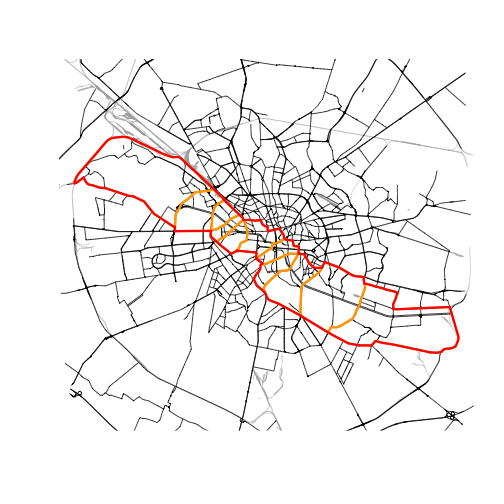

Interpretation and next steps

Use the segments and/or river spaces for comparative analyses along the river; or
Integrate relevant data layers within a segment and/or river space of interest; or
Run the analysis on other cities to compare a phenomenon of interest across corridors, segments and/or river spaces;
Export to GIS formats for further processing.

References

Forgaci, C. (2018). Integrated urban river corridors: Spatial design
for social-ecological integration in bucharest and beyond [PhD
thesis]. https://doi.org/10.7480/abe.2018.31