In a typical CRiSp workflow, valley delineation is used in the
context of corridor delineation. When the parameter
method = "valley" is set (this is the default value) in
delineate_corridor(), first the river valley is extracted
from a Digital Elevation Model (DEM) with
delineate_valley() and then the resulting valley edge is
used to “guide” the delineation of the corridor on the street network,
as shown in vignette("corridor-delineation").
In this article, we describe how delineate_valley()
works and how it can be used independently.
delineate_valley() uses a Cost Distance algorithm, variants
of which are mostly used for the delineation of wet area mapping and
valley bottom delineation in non-urban contexts (Ågren et al., 2014; Murphy et al., 2009; White et al.,
2012).
As the resulting valley boundary is only used as an intermediate step
in delineate_corridor(), valley delineation does not
require high-resolution DEM data, as required for non-urban applications
(e.g., Lidberg et al., 2020; Nardi et al.,
2019). By default, the valley is delineated on the openly
available 30m-resolution Copernicus
DEM GLO-30.
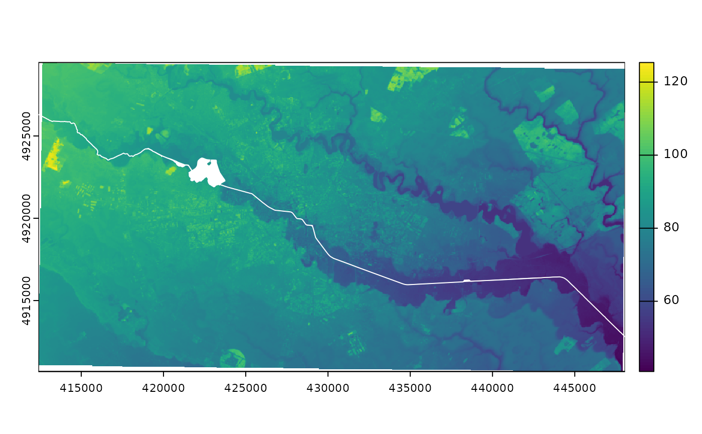
We demonstrate valley delineation using data from the CRiSpData package, namely the DEM of Bucharest as the input raster and the river centerline and surface as the source for which the Cost Distance is calculated.
# Attach required packages
library(CRiSp)
library(CRiSpData)
library(terra)
library(sf)

# Load data for valley delineation
dem <- unwrap(bucharest_dem)
river_centerline <- st_geometry(bucharest_osm$river_centerline)
river_surface <- st_geometry(bucharest_osm$river_surface)
river <- c(river_centerline, river_surface)
DEM of the area enclosing River Dâmbovița in Bucharest
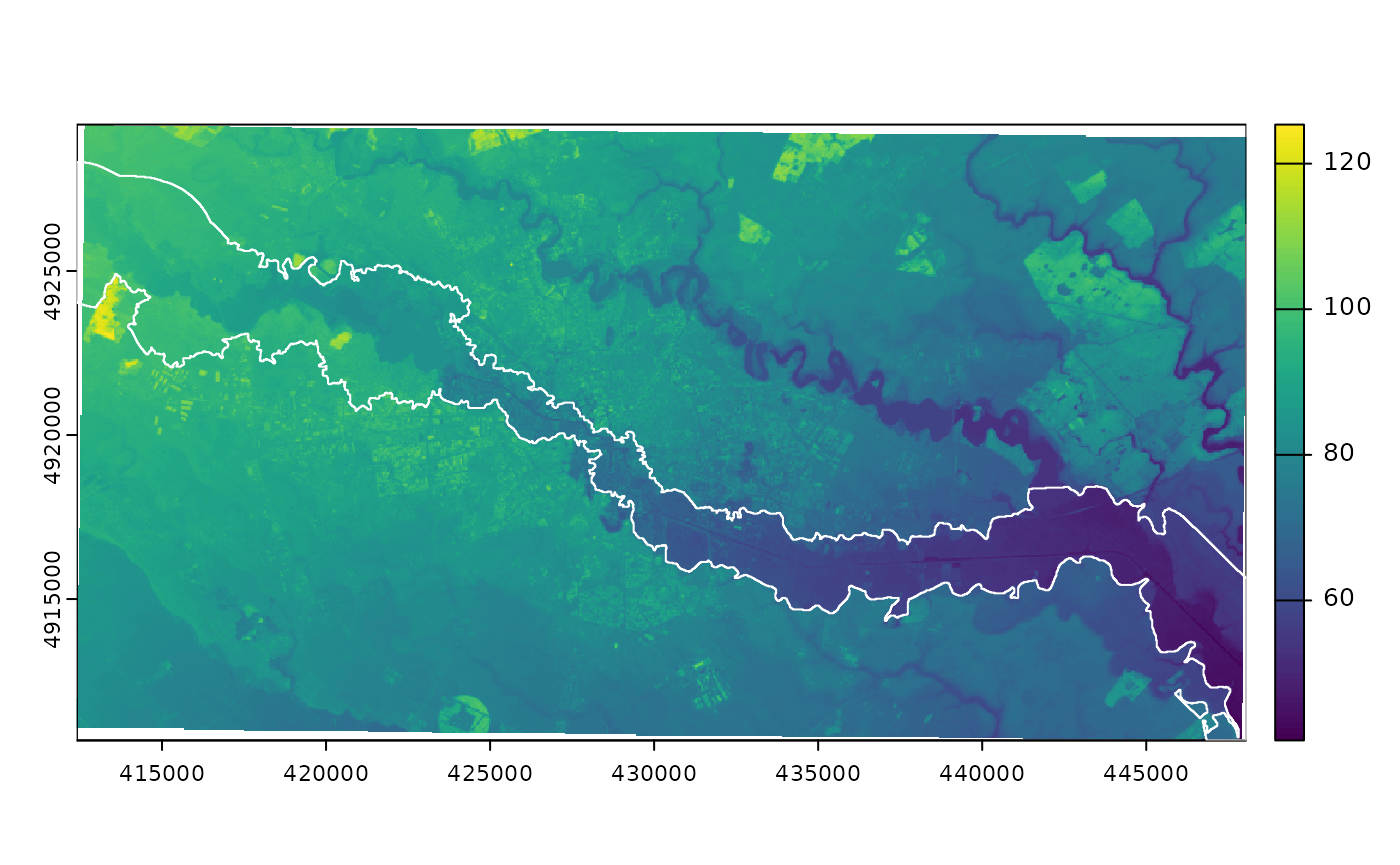
valley <- delineate_valley(dem, river)
Valley polygon derived from the DEM